The Algorithm with Adaptive Momentum

The goal is to choose minimization directions, which are not interfering and linearly independent. This can be achieved by the selection of conjugate directions which forms the basis of the CG method. Two vectors are non-interfering and linearly or mutually conjugate with respect to $\nabla ^2 E(w_t)$ when

$$dw_t ^T \nabla ^2 E(w_t) dw_{t-1} =0$$ (1025)

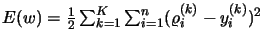
where $E(w)=\textstyle{\frac{1}{2}} \sum_{k=1}^K \sum_{i=1}^n (\varrho_i^{(k)}-y_i ^{(k)}) ^2$, $\nabla ^2 E(w_t)$ is the Hessian matrix $\mathbf{H}_t=\mathbf{J}^{{(k)}^T}\mathbf{J}^{(k)}+\mu^{(k)}\mathbf{I}$, with $K$ is the number of training patterns, $n$ is the number of outputs, $w_t$ the weights vector, and $dw_t$ is the optimal step (or the search direction). 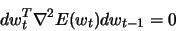The objective is to reach a minimum of the cost function with respect to $w_t$ and to simultaneously maximize 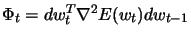$\Phi_t=dw_t^T \nabla ^2 E(w_t)dw_{t-1}$ without compromising the need for a decrease of the cost function. At each iteration of the learning process, the weight vector $w_t$ will be incremented by $dw_t$, so that:

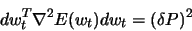$$dw_t ^T \nabla ^2 E(w_t) dw_{t} = (\delta P)^2$$ (1026)

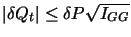
where $\delta P$ is a constant and the change $dE(w_t)$ in $E(w_t)$ is equal to a predetermined quantity $\delta Q_t < 0$:

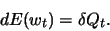$$dE(w_t)=\delta Q_t.$$ (1027)

This is a constrained optimization problem which can be analytically solved by introducing two Lagrange multipliers $\lambda_1$ and $\lambda_2$. Then function $\phi_t$ is introduced to evaluate the differentials involved in the right hand side and to substitute the function $\Phi_t$:

$$\phi _t =\Phi _t + \lambda _1 (\delta Q_t -dE(w_t)) +\lambda _2 [(\delta P)^2 -dw_t^T \nabla ^2 E(w_t) dw_t].$$ (1028)

By replacing $\Phi_t$ by its value, we obtain:

$$\phi _t = dw_t ^T\nabla ^2 E(w_t)dw_{t-1} +\lambda_1 (\de... ...w_t) +\lambda_2[(\delta P)^2 -dw_t^T \nabla ^2 E(w_t) dw_t].$$ (1029)

To maximize $\phi$ at each iteration, the following equations must be satisfied:

$$d\phi_t = d^2w_t^T(\nabla^2 E(w_t)dw_{t-1} -\lambda_1\nabla E(w_t)-2\lambda_2 \nabla^2E(w_t)dw_t)=0,$$ (1030)

and

$$d^2 \phi_t =-2\lambda_2[d^2w_t^T\nabla^2E(w_t)d^2w_t] < 0.$$ (1031)

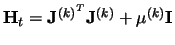
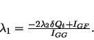
Hence from 10.30 we obtain:

$$dw_t =-\frac{\lambda_1}{2\lambda_2}[\nabla^2 E(w_t)]^{-1}\nabla E(w_t)+\frac{1}{2\lambda_2} dw_{t-1}.$$ (1032)

From equations 10.27 and 10.32 we obtain:

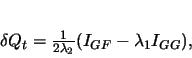$$\delta Q_t=\frac{1}{2\lambda_2} (I_{GF} -\lambda_1 I_{GG}),$$ (1033)

where

$$I_{GG}=\nabla E(w_t)^T [\nabla^2 E(w_t)]^{-1}\nabla E(w_t),$$ (1034)

$$I_{GF} =\nabla E(w_t)^T dw_{t-1}.$$ (1035)

From 10.33 we obtain $\lambda_1$:

$$\lambda_1=\frac{-2\lambda_2\delta Q_t +I_{GF}}{I_{GG}}.$$ (1036)

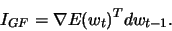
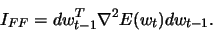
It remains to obtain $\lambda_2$. This can be done by substituting Eqn. 10.30 in Eqn. 10.26 to obtain:

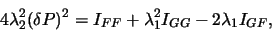$$4\lambda_2^2(\delta P)^2 =I_{FF}+\lambda_1 ^2 I_{GG} -2\lambda_1 I_{GF},$$ (1037)

where

$$I_{FF}=dw_{t-1} ^T \nabla^2 E(w_t)dw_{t-1}.$$ (1038)

Finally, Eqn. 10.36 is substituted into Eqn. 10.37 and solve for $\lambda_2$ to obtain:

$$\lambda_2=\textstyle \frac{1}{2} \displaystyle \left [ ... ...{I_{FF}I_{GG}-I_{GF}^2} \right]^{-\textstyle \frac{1}{2}}.$$ (1039)

The positive square root value has been chosen for $\lambda_2$ in order to satisfy Eqn. 10.31. Note the bound $\vert\delta Q_t\vert \leq \delta P \sqrt{I_{GG}}$ set on the value of $\delta Q_t$ by Eqn. 10.39. The value chosen for $\delta Q_t$ is always: $\delta Q_t = -\zeta \delta P \sqrt{I_{GG}}$ where $\zeta$ is a constant between 0 and 1. Therefore the free parameters are $\zeta$ and $\delta P$ ( $0< \delta P <1$). The authors recorded during their simulations that the best results are given for $0.85 \leq \zeta \leq 0.95$ and $0.1 \leq \delta P \leq 0.6$ .