Testing the Success Rate and the Performance

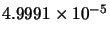
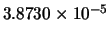
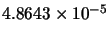
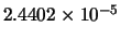
We have carried out two experiments to test the success rate and the performance of the training algorithms. To do that, for each training algorithm, we have fixed a MSE goal of $5\times 10^{-5}$ and $4\times 10^{-7}$ for the first and second problems respectively. It is known that the convergence of the NN training algorithms depends on the initial values of the weights, which are typically initialized randomly. We have thus repeated the same experiment for each problem and each training algorithm 100 times. We have limited the maximum number of iterations to 100. For each case, the random seed generator is fixed to the index of the test (from 1 to 100). This is to limit the biasing of the initialization on the comparison. The weights are initialized in the range 0 ...0.1. Each time the algorithm converges to the specified error, the delay and current error are stored. For each algorithm in the first and second problems, the success rate, the number of iterations statistics, the required time statistics, and the reached MSE statistics (the minimum, the maximum, the mean and the standard deviation) are calculated and reported. The results are shown in Tables 10.1 and 10.2 for the first and second problems respectively. For the AM-LM algorithm, we set $dP=0.6$ and $\zeta=0.90$. As we can see from Table 10.1, LM and GD give approximately the same success rate, but, LM converges in less iterations and time. The minimum and maximum time needed for LM are 0.33 and 3.58 with a mean of 1.15 sec. against 2.92 and 13.94 with a mean of 8.63 sec. for GD. However, when applying the non-negative weights constraint on LM, as shown in column LM2, the performance degrades too much. With respect to the AM-LM algorithm, it gives the best results among all the other algorithms. The success rate is 99. In addition, the required time and iterations are the best. The mean time needed is 0.67 against 8.63, 1.15, 14.25 sec. for GD, LM and LM2 respectively. We can note also that AM-LM can converge in only one iteration against 21, 2 and 48 iterations for GD, LM and LM2 respectively. Regarding the error, some times LM and AM-LM can converge to 0 error. It should be mentioned that AM-LM does not work well for the fully connected RNN network (as the case of the second problem). Thus, we do not provide the results in this case. We can note from Table 10.2 that LM converges all the times (100 successes). The convergence for GD is very poor, only 22 success rate. In addition, for LM without non-negative weights constraints, the results are better than all the other cases (LM1 and LM2). However, the performance is better than that of GD. LM can converge in only 5 iterations against 64, 9 and 38 iterations for GD, LM1 and LM2 respectively. Moreover, LM takes less time to converge (about 1.05 sec. in average against 9.56. 3.78 and 9.40 sec. for GD, LM1 and LM2 respectively). Similarly, the error statistics are minimal for LM. We can notice that both LM and AM-LM, when they converge, they do not take too much iterations (6 and 9 iterations for the first and second problems respectively). This can be used to improve the success rate and hence the performance by restarting the training using different weights initialization.

Table 10.1: Comparison between GD, LM, LM2 and AM-LM for the first problem.

	GD	LM	LM2	AM-LM
Success	81	83	50	99
Min(iterations)	21	2	48	1
Max(iterations)	97	24	100	6
Mean(iterations)	60.27	7.14	82.52	2.83
Std(iterations)	21.26	4.85	12.01	0.95
Min(time)(s)	2.92	0.33	8.4	0.22
Max(time)(s)	13.94	3.58	17.57	1.70
Mean(time)(s)	8.63	1.15	14.25	0.67
Std(time)	3.06	0.72	3.06	0.31
Min(error)	$3.0537\times 10^{-5}$	0	$4.7736 \times 10^{-5}$	0
Max(error)	$4.9987\times 10^{-5}$	$4.9293 \times 10^{-5}$	$4.9991 \times 10^{-5}$	$3.8730\times 10^{-5}$
Mean(error)	$4.8643\times 10^{-5}$	$2.4402\times 10^{-5}$	$4.9153 \times 10^{-5}$	$1.0993\times 10^{-6}$
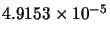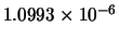Std(error)	$2.2703\times 10^{-6}$	$1.7641\times 10^{-5}$	$5.6558 \times 10^{-7}$	$5.0233\times 10^{-5}$

Table 10.2: Comparison between GD, LM, LM1 and LM2 for the second problem.

	GD	LM	LM1	LM2
Success	22	100	95	84
Min(iterations)	64	5	9	38
Max(iterations)	100	9	34	78
Mean(iterations)	86.45	5.48	18.51	56.32
Std(iterations)	11.76	0.88	4.93	9.27
Min(time)(s)	5.84	0.54	0.94	4.35
Max(time)(s)	9.56	1.05	3.78	9.40
Mean(time)(s)	8.14	0.67	2.05	6.69
Std(time)	1.12	0.10	0.53	1.17
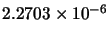
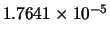
Min(error)	$3.3503\times 10^{-7}$	$4.6590\times 10^{-9}$	$5.3220\times 10^{-8}$	$2.8499\times 10^{-7}$
Max(error)	$3.9810\times 10^{-7}$	$3.8989\times 10^{-7}$	$3.9886\times 10^{-7}$	$3.9001\times 10^{-7}$
Mean(error)	$3.7638\times 10^{-7}$	$1.1062\times 10^{-7}$	$3.1342\times 10^{-7}$	$3.6046\times 10^{-7}$
Std(error)	$1.8052\times 10^{-8}$	$8.2365\times 10^{-8}$	$6.5777\times 10^{-8}$	$2.5932\times 10^{-8}$