Next: Descriptions of Our New
Up: Neural Networks
Previous: Artificial Neural Networks (ANN)
Contents
Index
Random Neural Networks (RNN)
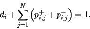
The Random Neural Networks (RNN) has been proposed by Erol Gelenbe in 1989 [45]. RNNs have been extensively studied, evaluated and analyzed in [49,89,48,45,101,51]; and analog hardware implementations of RNN are detailed in [3,25]. Low bit rate video compression using RNN is presented in [30]. A list of RNN applications are found in [2,4,6,7,50,99,123,128,148,10].
Gelenbe's idea can be described as a merge between the classical Artificial Neural Networks (ANN) model and queuing networks. Since this tool is a novel one, let us describe here its main characteristics. RNN are, as ANN, composed of a set of interconnected neurons. These neurons exchange signals that travel instantaneously from neuron to neuron, and send and receive signals to and from the environment. Each neuron has a potential associated with, which is an integer (random) variable. The potential of neuron  at time
  is denoted by
  . If the potential of neuron is strictly positive, the neuron is excited; in that state, it randomly sends signals (to other neurons or to the environment), according to a Poisson process with rate
  . Signals can be positive or negative. The probability that a signal sent by neuron goes to neuron
  as a positive one, is denoted by
  , and as a negative one, by
  ; the signal goes to the environment (that is, it leaves the network) with probability
  . So, if
  is the number of neurons, we must have for all
 ,
,
When a neuron receives a positive signal, either from another neuron or from the environment, its potential is increased by 1; if it receives a negative one, its potential decreases by 1 if it was strictly positive and it does not change if its value was 0. In the same way, when a neuron sends a signal, positive or negative, its potential is decreased by one unit (it was necessarily strictly positive since only excited neurons send signals)31.
The flow of positive (resp. negative) signals arriving from the environment to neuron (if any) is a Poisson process which rate is denoted by  (resp.
  ). It is possible to have
 and/or
 for some neuron , but to deal with an ``alive'' network, we need
 .
Finally, we make the usual independence assumptions between these arrival processes, the processes composed of the signals sent by each neuron, etc.
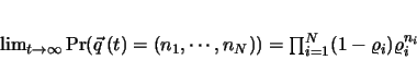
The discovery of Gelenbe is that this model has a product form stationary solution. This is similar to the classical Jackson's result on open networks of queues. If process
.
Finally, we make the usual independence assumptions between these arrival processes, the processes composed of the signals sent by each neuron, etc.
The discovery of Gelenbe is that this model has a product form stationary solution. This is similar to the classical Jackson's result on open networks of queues. If process
 is ergodic (we will say that the network is stable), Gelenbe proved that
 |
(31) |
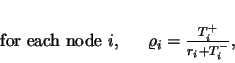
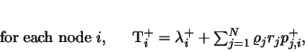
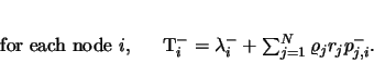
where the  s satisfy the following non-linear system of equations:
 |
(32) |
 |
(33) |
and
 |
(34) |
Relation (3.1) tells us that is the probability that, in equilibrium, neuron is excited, that is,
Observe that the non-linear system composed of equations (3.2), (3.3) and (3.4) has  equations and unknowns (the s, the
  s and the
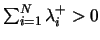
  s). Relations (3.3) and (3.4) tell us that is the mean throughput of positive signals arriving to neuron and that is the corresponding mean throughput of negative signals (always in equilibrium). Finally, Gelenbe proved, first, that this non-linear system has a unique solution, and, second, that the stability condition of the network is equivalent to the fact that, for all node ,
  .
Let us describe now the use of this model in statistical learning. Following previous applications of RNN, we fix the s to 0 (so, there is no negative signal arriving from outside). As a learning tool, the RNN will be seen as a black-box having inputs and outputs. The inputs are the rates of the incoming flows of positive signals arriving from outside, i.e. the s. The output values are the s. In fact, in applications, most of the time some neurons do not receive signals from outside, which simply corresponds to fixing some s to 0; in the same way, users often use as output only a subset of s.
At this point, let us assume that the number of neurons has been chosen, and that the topology of the network is selected; this means that we have selected the pairs of neurons that will exchange signals, without fixing the values of the rates and the branching probabilities and .
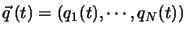
Our learning data is then composed of a set of
.
Let us describe now the use of this model in statistical learning. Following previous applications of RNN, we fix the s to 0 (so, there is no negative signal arriving from outside). As a learning tool, the RNN will be seen as a black-box having inputs and outputs. The inputs are the rates of the incoming flows of positive signals arriving from outside, i.e. the s. The output values are the s. In fact, in applications, most of the time some neurons do not receive signals from outside, which simply corresponds to fixing some s to 0; in the same way, users often use as output only a subset of s.
At this point, let us assume that the number of neurons has been chosen, and that the topology of the network is selected; this means that we have selected the pairs of neurons that will exchange signals, without fixing the values of the rates and the branching probabilities and .
Our learning data is then composed of a set of  input-output pairs, which we will denote here by
 , where
 and
and
 . The goal of the learning process is to obtain values for the remaining parameters of the RNN (the rates and the branching probabilities and ) such that if, in the resulting RNN, we set
 for all (and
 ), then, for all , the steady-state occupation probability is close to
  . This must hold for any value of
 .
To obtain this result, first of all, instead of working with rates and branching probabilities, the following variables are used:
.
To obtain this result, first of all, instead of working with rates and branching probabilities, the following variables are used:
This means that  (resp.
  ) is the mean throughput in equilibrium of positive (resp. negative) signals going from neuron to neuron . They are called
weights by analogy to standard ANN. The learning algorithm proceeds then formally as follows. The set of weights in the network's topology is initialized to some arbitrary positive value, and then iterations are performed which modify them. Let us call
) is the mean throughput in equilibrium of positive (resp. negative) signals going from neuron to neuron . They are called
weights by analogy to standard ANN. The learning algorithm proceeds then formally as follows. The set of weights in the network's topology is initialized to some arbitrary positive value, and then iterations are performed which modify them. Let us call
 and
and
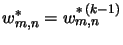
 the initial weights for the connection between and . Then, for
 , the set of weights at step
  is computed from the set of weights at step
  using a learning scheme, as usual with neural networks. More specifically, denote by
 the network obtained after step , defined by weights
 and
and
 . When we set the input rates (external positive signals) in
to the
. When we set the input rates (external positive signals) in
to the  s values, we obtain the steady-state occupations
 s (assuming stability). The weights at step are then defined by
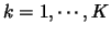
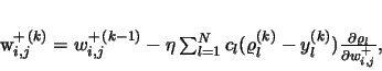 |
(35) |
 |
(36) |
where the partial derivatives
 (
( being `+' or `
 ') are evaluated at
 and
and
 .
Factor
.
Factor  is a cost positive term allowing to give different importance to different ouput neurons. If some neuron
  must not be considered in the output, we simply set
  . In our cases, we have only one output neuron, so, this factor is not relevant; we put it in (3.5) and (3.6) just to give the general form of the equation.
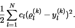
This is a gradient descent algorithm, corresponding to the minimization of the cost function
. In our cases, we have only one output neuron, so, this factor is not relevant; we put it in (3.5) and (3.6) just to give the general form of the equation.
This is a gradient descent algorithm, corresponding to the minimization of the cost function
Once again, the relations between the output and the input parameters in the product form result allows to explicitly derive a calculation scheme for the partial derivatives. Instead of solving a non-linear system as (3.2), (3.3) and (3.4), it is shown in [47] that here we just have a linear system to be solved. When relations (3.5) and (3.6) are applied, it may happen that some value
 or
or
 is negative. Since this is not allowed in the model, the weight is set to 0 and it is no more concerned by the updating process (another possibility is to modify the
  coefficient and apply the relation again; previous studies have been done using the first discussed solution, which we also adopt).
Once the learning values have been used, the whole process is repeated several times, until some convergence conditions are satisfied. Remember that, ideally, we want to obtain a network able to give output
coefficient and apply the relation again; previous studies have been done using the first discussed solution, which we also adopt).
Once the learning values have been used, the whole process is repeated several times, until some convergence conditions are satisfied. Remember that, ideally, we want to obtain a network able to give output
 when the input is
  , for .
As in most applications of ANN for learning purposes, we use a 3-level network structure: the set of neurons
, for .
As in most applications of ANN for learning purposes, we use a 3-level network structure: the set of neurons
 is partitioned into 3 subsets: the set of input nodes, the set of intermediate or hidden nodes and the set of output nodes. The input nodes receive (positive) signals from outside and don't send signals outside (that is, for each input node ,
 and
and  ). For output nodes, the situation is the opposite:
and
). For output nodes, the situation is the opposite:
and  . The intermediate nodes are not directly connected to the environment; that is, for any hidden neuron , we have
 . Moreover, between the nodes inside each level there are no transitions. Last, input neurons are only connected to hidden ones, and hidden neurons are only connected to output ones.
This is a typical structure for neural networks used as a learning tool. Moreover, RNN mathematical analysis (that is, solving the non-linear and linear systems) is considerably simplified in this case. In particular, it can easily be shown that the network is always stable. See [47] or [46] and Chapter 10 for the details.
ChapterChapter
. Moreover, between the nodes inside each level there are no transitions. Last, input neurons are only connected to hidden ones, and hidden neurons are only connected to output ones.
This is a typical structure for neural networks used as a learning tool. Moreover, RNN mathematical analysis (that is, solving the non-linear and linear systems) is considerably simplified in this case. In particular, it can easily be shown that the network is always stable. See [47] or [46] and Chapter 10 for the details.
ChapterChapter
Next: Descriptions of Our New
Up: Neural Networks
Previous: Artificial Neural Networks (ANN)
Contents
Index
Samir Mohamed
2003-01-08